Categories
Tutorials

Single Imputation using the Expectation-Maximization Algorithm

In this post, I outline when and how to use single imputation using an expectation-maximization algorithm in SPSS to deal with missing data. I start with a step-by-step tutorial on how to do this in SPSS, and finish with a discussion of some of the finer points of doing this analysis.

1. Open the data-file you want to work with.

2. Sort the data file by ascending ID or Participant number. This is critical; if you do not do this, everything you do subsequently could be inaccurate. To do this, right click on the ID column, and click “sort ascending”

EM1

3. Open the Syntax Editor in SPSS:

EM2

4. Copy and paste the following syntax into the Syntax Editor, adding in your own variables after MVA VARIABLES, and specifying a location on your computer after OUTFILE. .Also, note that .sav is the file extension for an SPSS file, so make sure it ends in that.

MVA VARIABLES=var1 var2 var3 var4 var5

/MPATTERN

/EM(TOLERANCE=0.001 CONVERGENCE=0.0001 ITERATIONS=100 OUTFILE=’C:\Users\Owner\Desktop\file1.sav’).

5. Highlight all the text in the syntax file, and click on the “run” button on the toolbar:

EM3

6. This will produce a rather large output file, but only a few things within are necessary for our purposes: (a) Little’s MCAR Test and (b) whether or not the analysis converged. Both can be found in the spot indicated in the picture below:

EM4

(a) If Little’s MCAR test is nonsignificant, this is a good thing! It means that your variables are missing Completely at Random (see #4 in FAQ).

(b) This second message is an error. It will only pop up if there is a problem. If you don’t find it at all in the output, it’s because everything is working properly. If this message DOES pop up, it means that the data imputation will be inaccurate. To fix it, increase the number of iterations specified in the syntax (e.g. try doubling it to 200 first). If that doesn’t work, try reducing the number of variables in your analysis.

9. The syntax you ran also saved a brand new datafile in a location you specified above. Open that datafile.

10. If everything went well, this new data file will have no missing data! (You can verify this for yourself by running analyzeàFrequencies on all your variables). However, the new datafile will ONLY contain the variables listed in the syntax above. If you want to have these variables in your master data file, you will have to merge the files together.

 Merging the master file and the file created with EM above

11. In the data file created with the above syntax, rename every variable. Make it simple, something like the following syntax:

RENAME VARIABLES (var1 = var1_em).

You are doing this because you do not want to overwrite the raw data with missing values included in the master data file.

12. Next, add an ID number variable (representing the participant ID number) that will be identical to whatever is in your master file (including variable name!). You’ll need this later to merge the files. If you sorted correctly, you should be able to copy and paste it from the master file.

13. Make sure both the master data file and the new data file created with the above syntax are open at the same time. Make sure both files are sorted by ascending ID number, as described in step 2. I can’t stress this enough. Double check to make sure you have done this.

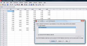
14. In the master file (not the smaller, newly-created file), Click on Data –> Merge Files –> Add Variables

EM10

15. Your new data set should be listed under “open datasets.” Click on it and press “continue”

EM11

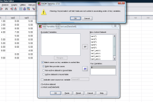
16. In the next screen, click “match cases on key variables in sorted files,” and “Both files provide cases.” Place “ID” (or whatever your participant ID number variable is) in the box “key variables.” Then click okay. You will get a warning message; if you sorted the data files by ID number as instructed, you may click “ok” again to bypass the warning message.

EM16

17. The process is complete! You now have a master dataset with a set of variables with the missing data replaced as well as the raw data with the missing data still included. This is valuable to make sure that you aren’t getting drastically different results between the imputed data and listwise deletion. When conducting your analyses, just make sure to use the variables that have no missing data!

FAQ

1. How does the EM Algorithm impute missing data?

Most of the texts on this topic are very complex and difficult to follow. After much searching on the web, I found a useful website which explains the conceptual ideas of EM in a very easy-to-understand format (http://www.psych-it.com.au/Psychlopedia/article.asp?id=267). So check this website out if you want to know what’s going on “under the hood.”

2. When should I use EM?

Generally speaking, multiple imputation (MI) and the full-maximum likelihood (FIML) methods are both less biased, and in the case of FIML, quicker to implement. Use those methods wherever possible. However, sometimes the EM approach is useful when you want to create a single dataset for exploratory analysis, and the amount of missing data is trivial. It’s also sometimes useful to overcome software limitations at the analysis stage. For example, bootstrapping cannot be performed in AMOS software with missing data using the default FIML approach. Moreover, there is often no agreed-upon way to combine results across multiply imputed datasets for many statistical tests. In both of these cases, a single imputation using EM may be helpful.

As a rule of thumb, only use EM when missing data are less than 5%. If you have more missing data than this, your results will be biased. Specifically, the standard errors will be too low, making your p-values too low (increasing Type I error).

3. Which variables should I include in my list when imputing data?

This is a tricky question. If you read tutorial on EM in #1 above, you will have an understanding that the EM algorithm imputes missing data by making a best estimate based on the available data. Long story short, if none of your variables are intercorrelated, you can’t make a good prediction using this method. Here are a few tips to improve the quality of the imputation:

a) Though it’s tempting to just throw in all of your variables, this isn’t usually the best approach. As a rule of thumb, do this only when you have 100 or fewer variables and a large sample size (Graham, 2009).

b) If you’re doing questionnaire research, it’s useful to impute data scale by scale. For instance, with an 8-item extraversion scale, run an analysis with just those 8 items. Then run a separate analysis for each questionnaire in a similar fashion. Merging the data files together will be more time-consuming, but it may provide more accurate imputations.

c) If you want to improve the imputation even further, add additional variables that you know are highly correlated (r > .50) with your questionnaire items of interest. For example, if you have longitudinal data where the same variable is measured multiple times, consider including the items from each wave of data when you’re imputing data. For instance, include the 10 items from time 1 depression and the 10 items from time 2 depression for a total of 20 items.

4. What does Little’s MCAR test tell us?

Missing data can be Missing Completely at Random (i.e., no discernible pattern to missingness), Missing at Random (i.e., missingness depends upon another observed variable), or Missing Not At Random (i.e., missingness is due to some unmeasured variable). Ideally, missing data should be Missing Completely at Random, as you’ll get the least amount of bias. A good tutorial on this distinction can be found in Graham (2009).

Littles MCAR test is an omnibus test of the patterns in your missing data. If this test is non-significant, there is evidence that your data are Missing Completely At Random. Be aware though, that it doesn’t necessarily rule out the possibility that data are Missing at Random – after all, if the variable wasn’t in the model, you’ll never know if it was important.

5. How might I report this missing data strategy in a paper?

I suggest something like the following:

“Overall, only 0.001% of items were missing from the dataset. A non-significant Little’s MCAR test, χ2(1292) = 1356.62, p = .10, revealed that the data were missing completely at random (Little, 1988). When data are missing completely at random and only a very small portion of data are missing (e.g. less than 5% overall), a single imputation using the expectation maximization algorithm provides unbiased parameter estimates and improves statistical power of analyses (Enders, 2001; Scheffer, 2002). Missing data were imputed using Missing Values Analysis within SPSS 20.0

Supplementary Resources

Enders, C. K. (2001). A primer on maximum likelihood algorithms available for use with missing data. Structural Equation Modeling, 8, 128-141. doi: 10.1207/S15328007SEM0801_7

Graham, J. W. (2009). Missing data analysis: Making it work in the real world. Annual Review of Psychology, 60, 549-576. doi: 10.1146/annurev.psych.58.110405.085530

Scheffer, J. (2002). Dealing with missing data. Research Letters in the Information and Mathematical Sciences, 3, 153-160. Retrieved from http://equinetrust.org.nz/massey/fms/Colleges/College%20of%20Sciences/IIMS/RLIMS/Volume03/Dealing_with_Missing_Data.pdf

Categories
Tutorials

Four Simple SPSS Syntax Tips

Here are four useful tips for writing shorter, more efficient SPSS syntax.

1. A simpler way to calculate scale totals.

I often need to calculate a total score for questionnaires with multiple items. For example, I might ask participants to answer ten different questions, responding to each question using a scale of 1 (strongly disagree) to 5 (strongly agree). In particular, I’ll often want to calculate an average of all ten items to use in statistical analyses. I used to calculate scale totals using the following SPSS syntax:

[box] COMPUTE vartotal = (var1 + var2 + var3 + var4 + var5 + var6 + var7 + var8 + var9 + var10) / 10.
EXECUTE.[/box]

So, this would create one new variable “vartotal” which would be the average of all 10 items. A quicker way to do this would be:

[box]MEAN(Var1 TO Var10).
EXECUTE.[/box]

There are two important caveats to keep in mind when using the quicker syntax.

First, variables need to be arranged side-by-side in columns in your database for the “TO” command to work properly. In the above example using the TO command, the syntax takes the average of Var1, Var10 and every variable in between. So if there were other, unwanted variables in between Var1 and Var10 in your dataset (e.g., maybe it went var1, var2, var3, sex, var4 …), SPSS won’t know that you didn’t want those extra variables, and will just average them all together.

Second, these two approaches handle missing data in a slightly different way. The first example I provided will return a “system missing” value for vartotal if there is ANY missing data on any of the 10 individual items. In contrast, the second shorter syntax example will report the mean of all existing variables (e.g., if you were missing a value for var5, SPSS would add the remaining 9 items together and divide by 9). Depending on how you plan on dealing with missing data, this could be undesirable.

2. A shorter way to reverse-score items

Another thing I often need to do when working with questionnaires is reverse-scoring. For example, I might have these two items:

“Is talkative”
“Tends to be quiet”

These two items are measuring the same thing (Extraversion), but are worded in the opposite way. If I want high values of the total score to indicate high levels of Extraversion, I would reverse code “tends to be quiet” so that low values are now high, and vice versa. So, assuming that this was measured on a 9-point scale from 1 (strongly disagree) to 9 (strongly agree), one way to do this would be:

[box]RECODE var1 (1=9) (2=8) (3=7) (4=6) (5=5) (6=4) (7=3) (8=2) (9=1) INTO var1_r.
EXECUTE.[/box]

That can be a little tedious to write out, so an alternative would be the following:

[box]COMPUTE Var1_r=ABS(Var1 – 10).
EXECUTE.[/box]

In this syntax, I take the absolute value of Var1 – 10. You will always subtract a number 1 higher than the highest possible value on your scale.

3. Saving a smaller datafile with only a subset of variables

If you’re working on really large datasets, sometimes you want to create a dataset that contains only a handful of variables that you’re interested in (e.g., the full dataset has 1000 variables, but you only care about 5 of them). There’s a very simple bit of syntax that will let you do this with ease:

[box]SAVE OUTFILE=’C:\Users\Sean Mackinnon\Desktop\small_data.sav’
/KEEP= var1 var2 var3 var4 var5
/COMPRESSED.[/box]

This will create a new datafile that contains only the five variables you specified, deleting all the rest. I find this to be very useful when dealing with enormous datasets.

4. The COUNT command: Counting the number of instances of a particular value

Occasionally, I need to count the frequency of a particular response. For example, when measuring alcohol consumption, I might have 7 variables: drinkday1 TO drinkday7. Each of these variables indicates how many alcoholic beverages a person had on a particular day.

What if I want to know how many days participants had did not drink at all? This can be easily done with the COUNT command in SPSS:

[box]COUNT drinkfreq = drinkday1 TO drinkday7 (0).
EXECUTE.[/box]

The above syntax will look at all seven days (i.e., drinkday1 TO drinkday7), and count the number of “0” values for each participant. So if a single participant had these values:

drinkday1 = 1
drinkday2 = 0
drinkday3 = 0
drinkday4 = 0
drinkday5 = 7
drinkday6 = 2
drinkday7 = 3

The above syntax would report a value of “3” because on three of those days, the participant had zero drinks.

What if I want to know how many days participants had at least one drink? We could accomplish this with similar syntax:

[box]COUNT drinkfreq = drinkday1 TO drinkday7 (1 THRU 100).
EXECUTE.[/box]

In this case, we’re counting all the instances of values from 1 to 100 (assuming that nobody has more than 100 drinks in a day!). So using the same data as above, this time the count command would produce a value of “4.” The count command is pretty flexible, and is useful for this kind of problem.

Hopefully you find some of these useful! Feel free to post a comment if anything is unclear.

[facebook]

Categories
Tutorials

Converting an SPSS datafile to Mplus format

Converting an SPSS datafile into a format readable by Mplus

Mplus  is a fabulous statistical program. It’s very flexible, and is my favorite program to use when I need to analyze data using structural equation modeling – and I definitely prefer it over AMOS software. The latter is easier to use because of the graphical user interface (GUI), but I often find myself running into software limitations (e.g., AMOS cannot use bootstrapping when there is missing data) and in complex models, I often find the GUI tends to get clunky, and visually cluttered. This said, Mplus is not terribly user-friendly for new users – despite having an extensive discussion board of answers to various problems.

Much of my initial training – like many in psychology – was running statistics using SPSS software. SPSS has the advantage of being very user friendly, but moving to a syntax-based coding language like the one used by Mplus can be daunting at first. When I was first trying to figure out Mplus for myself during graduate school, I immediately ran into a problem: The datafile I had was not properly formatted for Mplus. Since (at the time) I had been mostly working with SPSS software, my datafile was in .sav format (the proprietary format of SPSS). Before I could get started, I needed to convert the file into format understandable by Mplus. Sounds simple, right? Well, it is actually. But the problem is that there is a LOT of documentation on Mplus, and finding precisely what needs to be done to your dataset to get started isn’t immediately apparent.  With this in mind, I’m going to present three simple steps to convert your SPSS datafile into a form readable by Mplus.

Step 1: Make sure missing values are indicated by a specific value

If you’re an SPSS user, you may be used to leaving missing values as “blanks” within SPSS itself. What may not be immediately apparent is that SPSS still needs to indicate missing values with a character of some sort. Specifically, SPSS actually fills in any blanks with a period (.) by default, and designates all periods as a piece of missing data. If you look closely at your SPSS datafile when it’s open, you can actually see the periods filled in all for the blanks.

Unfortunately, Mplus doesn’t like it when you use periods as the symbol for missing data. Even though Mplus can ostensibly use periods as missing data indicators, I would recommend that you pick some other number to represent missing data. When I was first working with Mplus using periods as missing data indicators, I kept getting incredibly uninformative error messages (or alternatively, the program would sometimes instead read the data incorrectly without giving an error message) which I eventually figured out was being caused by having my missing values represented by a period, as is default in SPSS. I usually use “999” to represent missing data instead. You can replace all the periods with “999’s” this very easily in SPSS using the following syntax:

[box] RECODE var1 var2 var3 var4 var5 (SYSMIS=999) (ELSE=COPY). EXECUTE.[/box]

Step 2: Rename variables to be 8 characters or less

Though this is technically optional, Mplus will truncate all variable names to 8 characters in your output.  So unless you want to be really confused later when running your analyses, I recommend that you assign new variable names to all your variables that 8 characters or less. For example, if your variable was “self_esteem_academic,” Mplus would shorten that to just “self_est” in the output. A better variable name might be something like “se_a.” In case you want to do this multiple times, you might write syntax to do this instead of changing all the variable names manually in the variable viewer:

[box] RENAME VARIABLES (longvariable1 longvariable2 = var1 var2). EXECUTE. [/box]

Step 3: Convert the file into fixed-format ASCII

For Mplus to work its magic, your datafile needs to be in fixed-format ASCII.  All you really need to know is that fixed-format ASCII files have the data arranged in columns with fixed sizes so that every record fits into a standard form (as opposed to, say, comma-delimited format, where each field is separated or ‘delimited’ by a comma). To convert an SPSS file (.sav) into fixed-format ASCII, first go into “variable view” and make sure that the “columns” and “width” columns in SPSS are all the same number. This is going to determine the space in between columns. If you were to pick a number like “12” it should be good for most purposes (unless you have very large numbers, or need many decimal places of precision).  Instead of doing this manually, there is a straightforward kind of syntax that can alter the column widths of all your variables:

[box]*f = numeric, 12 = column width, .0 = decimals) ALTER TYPE var1 TO var10 (f12.0). EXECUTE. [/box]

After you do this, open up your SPSS file and run the following syntax:

[box] WRITE OUTFILE=’C:\FileLocation\datafile_formplus.dat’ TABLE /ALL. EXECUTE.[/box]

Yup, it’s that straightforward. Before getting too far into your analyses, I would also recommend that you do some basic diagnostics by running simple analyses in both programs (e.g., checking means and standard deviations in SPSS and Mplus) to make sure that the conversion worked as expected. Note also that a fixed-format ASCII file doesn’t have variable names listed on the top! They will be in the same order as they were in the SPSS file, but this is another area where you might get confused when starting to run analyses (in every Mplus syntax file, you will list all the variables in order; if you make a mistake in that list though, your analyses will be wrong!). Aside from that though, you should be good to start analyzing data in Mplus!

****Update: Feb 16, 2015****

A reader helpfully pointed out that in version SPSS version 22, there is a problem that requires an additional step. For some reason, version 22 adds some nonsense characters to the beginning of the file that prevents Mplus from reading it. In order to work around this, you will have to open up the saved datafile in the Mplus Editor, and delete the characters manually. Annoyingly, these characters won’t show up if you open the datafile in notepad, excel, or SPSS, so you have to open it in the Mplus editor to find and delete them! Below is a picture showing the problem, and indicating what characters you need to delete. This should only be required if you have SPSS version 22, earlier versions do not require this workaround — when I originally wrote this tutorial, I used SPSS 20, which didn’t have this problem!

mplus.character

[facebook]

Categories
Tutorials

The Three Most Common Types of Hypotheses

Simple main effects (i.e., X leads to Y) are usually not going to get you published. Main effects can be exciting in the early stages of research to show the existence of a new effect, but as a field matures the types of questions that scientists are trying to answer tend to become more nuanced and specific.  In this post, I’ll briefly describe the three most common kinds of hypotheses that expand upon simple main effects – at least, the most common ones I’ve seen in my research career in psychology – as well as providing some resources to help you learn about how to test these hypotheses using statistics.

Incremental Validity

“Can X predict Y over and above other important predictors?”

Inc_Validity

This is probably the simplest of the three hypotheses I propose. Basically, you attempt to rule out potential confounding variables by controlling for them in your analysis.  We do this because (in many cases) our predictor variables are correlated with each other. This is undesirable from a statistical perspective, but is common with real data. The idea is that we want to see if X can predict unique variance in Y over and above the other variables you include.

In terms of analysis, you are probably going to use some variation of multiple regression or partial correlations.  For example, in my own work I’ve shown in the past that friendship intimacy as coded from autobiographical narratives can predict concern for the next generation over and above numerous other variables, such as optimism, depression, and relationship status (Mackinnon et al., 2011).

Moderation

“Under what conditions does X lead to Y?”

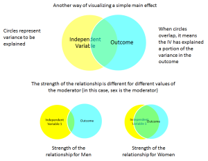
Of the three techniques I describe, moderation is probably the most tricky to understand.  Essentially, it proposes that the size of a relationship between two variables changes depending upon the value of a third variable, known as a “moderator.”  For example, in the diagram below you might find a simple main effect that is moderated by sex. That is, the relationship is stronger for women than for men:

moderation

With moderation, it is important to note that the moderating variable can be a category (e.g., sex) or it can be a continuous variable (e.g., scores on a personality questionnaire).  When a moderator is continuous, usually you’re making statements like: “As the value of the moderator increases, the relationship between X and Y also increases.”

Mediation

“Does X predict M, which in turn predicts Y?”

We might know that X leads to Y, but a mediation hypothesis proposes a mediating, or intervening variable. That is, X leads to M, which in turn leads to Y.  In the diagram below I use a different way of visually representing things consistent with how people typically report things when using path analysis.

Mediation

I use mediation a lot in my own research. For example, I’ve published data suggesting the relationship between perfectionism and depression is mediated by relationship conflict (Mackinnon et al., 2012). That is, perfectionism leads to increased conflict, which in turn leads to heightened depression. Another way of saying this is that perfectionism has an indirect effect on depression through conflict.

Helpful links to get you started testing these hypotheses

Depending on the nature of your data, there are multiple ways to address each of these hypotheses using statistics. They can also be combined together (e.g., mediated moderation). Nonetheless, a core understanding of these three hypotheses and how to analyze them using statistics is essential for any researcher in the social or health sciences.  Below are a few links that might help you get started:

Are you a little rusty with multiple regression? The basics of this technique are required for most common tests of these hypotheses. You might check out this guide as a helpful resource:

https://statistics.laerd.com/spss-tutorials/multiple-regression-using-spss-statistics.php

David Kenny’s Mediation Website provides an excellent overview of mediation and moderation for the beginner.

http://davidakenny.net/cm/mediate.htm

http://davidakenny.net/cm/moderation.htm

Preacher and Haye’s INDIRECT Macro is a great, easy way to implement mediation in SPSS software, and their MODPROBE macro is a useful tool for testing moderation.

http://afhayes.com/spss-sas-and-mplus-macros-and-code.html

If you want to graph the results of your moderation analyses, the excel calculators provided on Jeremy Dawson’s webpage are fantastic, easy-to-use tools:

http://www.jeremydawson.co.uk/slopes.htm

[facebook]